How least-squares fitting works
This page explains what happens when you call fit(). The math is kept
to what you need to read a fit result intelligently. No background in
optimisation is assumed.
If you just want to run a fit, start with the Quickstart.
1. What is a residual?
Every data point is a measurement \((x_i, y_i)\) with uncertainty \(\sigma_i\). We choose a model \(M(x; \boldsymbol{\theta})\) with adjustable parameters \(\boldsymbol{\theta}\). For a straight line the parameters are \(\boldsymbol{\theta} = [m, c]\) and \(M(x) = m x + c\).
The residual is the difference between the measured value and the model prediction:
A good fit makes all the residuals small.
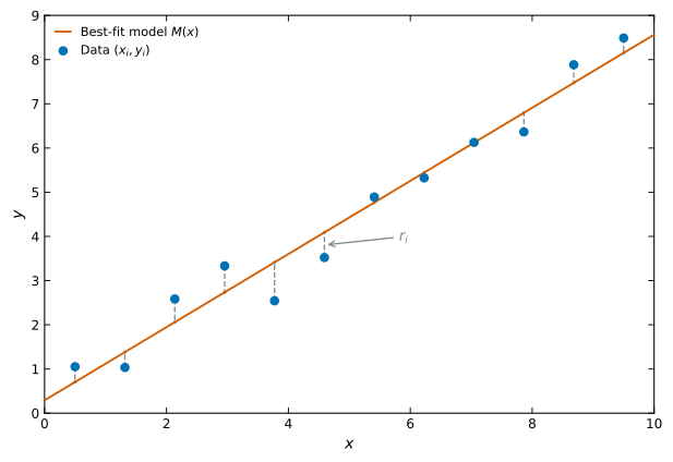
Each dashed vertical line is a residual: the distance from the data point to the fitted curve.
2. Why square the residuals?
Adding residuals directly lets positive and negative values cancel. We could take absolute values (\(\sum |r_i|\)), but squaring has two advantages:
Large deviations are penalised more than small ones. A point twice as far from the curve contributes four times as much to the cost.
The squared sum is differentiable, which lets us use calculus to find the best parameters efficiently.
Define the objective function (also called the cost):
Dividing by \(\sigma_i^2\) means points with large uncertainties matter less than points with small ones.
3. The \(\chi^2\) landscape
For a two-parameter model like a straight line, every pair \((m, c)\) produces a \(\chi^2\) value. Plotting \(\chi^2\) against the parameters gives a surface.
For linear models (line, polynomial) the surface is a perfect parabola with one global minimum.
For nonlinear models (Gaussian, exponential) the surface can be bumpy with local minima and ridges.
Finding the best-fit parameters means sliding downhill on this surface until you reach the bottom.
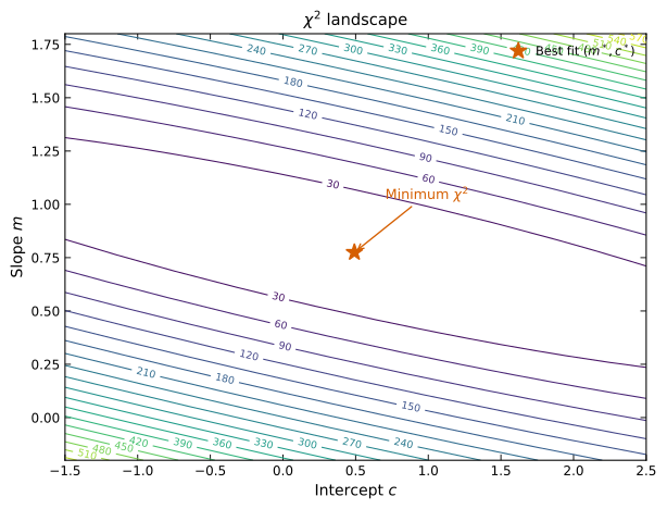
Each contour connects parameter pairs with the same \(\chi^2\). The star marks the minimum: the best-fit parameters.
4. How the optimiser walks downhill
The surface shows the destination. The optimiser is the algorithm that
gets you there. LabFit uses SciPy’s least_squares with the Trust Region
Reflective (TRF) method. The idea is the same for any gradient-based
method:
Start somewhere with an initial guess \(\boldsymbol{\theta}_0\) (supplied via
p0or from automatic heuristics).Look at the local slope by computing the gradient of \(\chi^2\) with respect to each parameter.
Take a step downhill in the direction that reduces \(\chi^2\) most.
Repeat until the gradient is nearly zero or improvement stalls.
The TRF method goes further. It builds a local quadratic model of the
surface (a “trust region”) to pick better step sizes. It also respects
parameter bounds: if you set amplitude to be positive, the optimiser
never tries negative values.
5. Goodness-of-fit: reduced \(\chi^2\)
Once the optimiser finds the minimum \(\chi^2_{\min}\), we compute the reduced chi-square:
where \(N\) is the number of data points and \(k\) is the number of free parameters. The denominator is the degrees of freedom.
The reduced \(\chi^2\) tells you whether your model and your uncertainties are consistent:
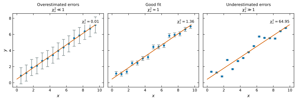
Same data-generating process but different reported uncertainties produce different \(\chi^2_\nu\) values.
\(\chi^2_\nu \approx 1\) means the scatter matches the error bars.
\(\chi^2_\nu \gg 1\) means the data scatter more than the error bars suggest. The model may be too simple, uncertainties may be underestimated, or there may be outliers.
\(\chi^2_\nu \ll 1\) means the scatter is smaller than expected. The error bars may be overestimated.
LabFit also returns a p-value for a more formal test. A very small p-value (below 0.01) suggests the model is a poor description of the data.
6. Parameter uncertainties
The best-fit parameters are only part of the result. We also need to know how confident we are in each value. That information comes from the shape of the \(\chi^2\) surface at the minimum.
If the \(\chi^2\) valley is steep and narrow in a particular direction, that parameter is tightly constrained. Small changes increase the cost a lot, so the uncertainty is small.
If the valley is shallow and flat, the parameter can vary widely without changing \(\chi^2\) much. Its uncertainty is large.
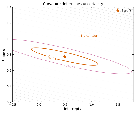
The \(\chi^2_{\min}+1\) contour encloses the 1-\(\sigma\) confidence region. A steep valley means a small uncertainty; a flat valley means a large uncertainty.
The covariance matrix \(C\) captures this curvature:
where \(J\) is the Jacobian (the gradient of the residuals with respect
to the parameters) at the best fit. The parameter uncertainties in
result.uncertainties are the square roots of the diagonal entries:
For more detail on reduced \(\chi^2\) and error propagation, see Concepts: reduced χ² and error propagation. For the full API reference, see API Reference.