Gallery
The examples below are fully reproducible and the accompanying images are
committed under docs/_static/gallery/. They are generated from the same
public API you would use in your own analysis.
Linear fit with residuals
This example shows the core least-squares flow from raw arrays to a fit result with uncertainties and residuals.
import numpy as np
from labfit import fit_curve, plot_fit

rng = np.random.default_rng(20240606)
x = np.linspace(0.0, 8.0, 30)
sigma = 0.10 + 0.02 * (1.0 + np.sin(x))
y = 1.85 * x - 0.65 + rng.normal(0.0, sigma)

result = fit_curve("linear", x, y, sigma)
plot = plot_fit(result, show_residuals=True, title="Linear fit with residuals")
plot.save("docs/_static/gallery/linear_fit.png")
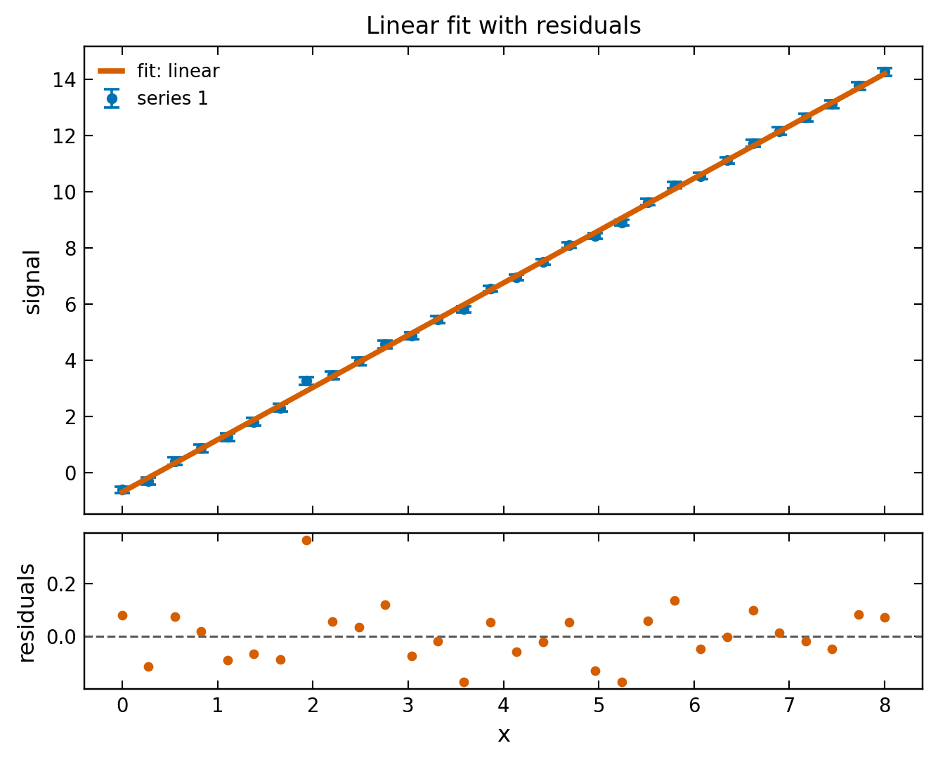
Least-squares line fit with a residual panel underneath.
Linear fit console output
slope = 1.860589 ± 0.008830
intercept = -0.694920 ± 0.041056
reduced chi^2 = 0.788588
Gaussian fit
This example uses the built-in Gaussian model with automatic initial guesses.
import numpy as np
from labfit import fit, plot_fit

rng = np.random.default_rng(20240607)
x = np.linspace(-5.0, 5.0, 260)
y = 4.0 * np.exp(-0.5 * ((x - 0.75) / 1.10) ** 2) + 0.18
y = y + rng.normal(0.0, 0.08, size=x.size)

result = fit(x, y, model="gaussian")
plot = plot_fit(result, show_residuals=True, title="Gaussian fit")
plot.save("docs/_static/gallery/gaussian_fit.png")
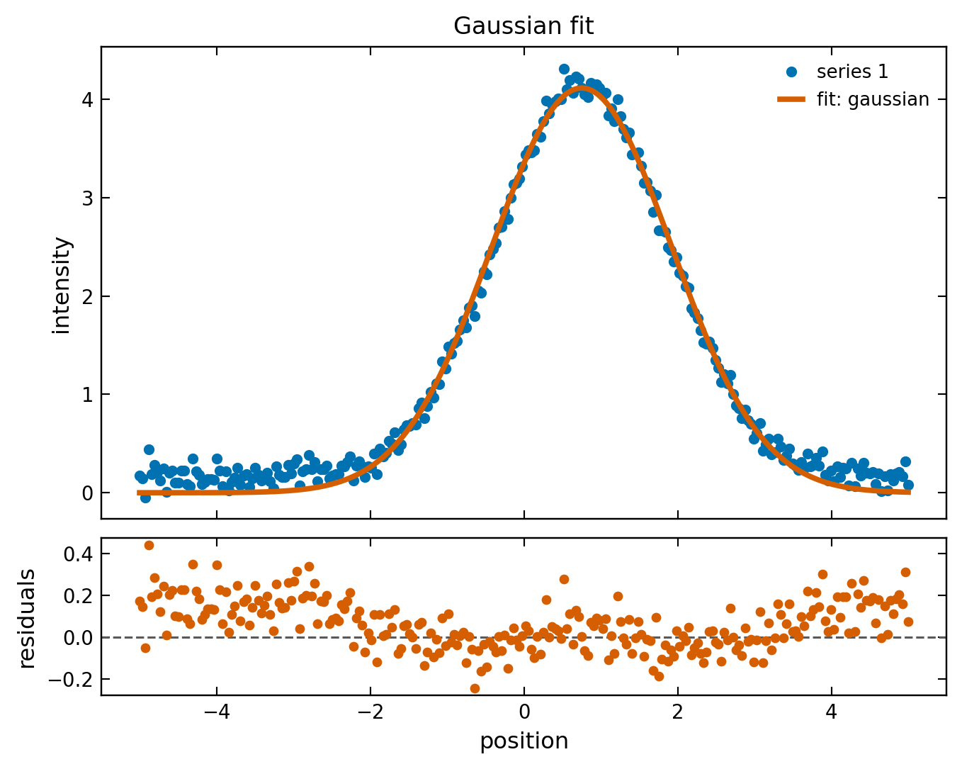
A standard Gaussian fit using the built-in model and automatic initial guess.
Gaussian fit console output
amplitude = 4.1157361 ± 0.0221282
mean = 0.7529858 ± 0.0072789
sigma = 1.1724581 ± 0.0072790
reduced chi^2 = 0.0175698
Multi-series damped oscillator comparison
This example shows labfit.fit_multi() and labfit.plot_multi_fit() on
paired experimental series.
import numpy as np
from labfit import Fitter, Series, plot_multi_fit

def damped_oscillator(t, amplitude, damping, f, phase):
    return amplitude * np.exp(-damping * t) * np.cos(2.0 * np.pi * f * t + phase)

rng = np.random.default_rng(20240608)
x1 = np.linspace(0.0, 6.0, 240)
x2 = np.linspace(0.0, 6.0, 220)
s1 = Series(x=x1, y=damped_oscillator(x1, 1.25, 0.22, 0.98, 0.10) + rng.normal(0, 0.03, size=x1.size), sigma=0.03, label="Trial 1")
s2 = Series(x=x2, y=damped_oscillator(x2, 1.05, 0.18, 1.02, -0.05) + rng.normal(0, 0.03, size=x2.size), sigma=0.03, label="Trial 2")

fitter = Fitter(model=damped_oscillator, p0={"amplitude": 1.0, "damping": 0.2, "f": 1.0, "phase": 0.0})
results = fitter.fit_multi([s1, s2])
plot = plot_multi_fit(results, [s1, s2], title="Damped oscillator comparison")
plot.save("docs/_static/gallery/damped_oscillators.png")
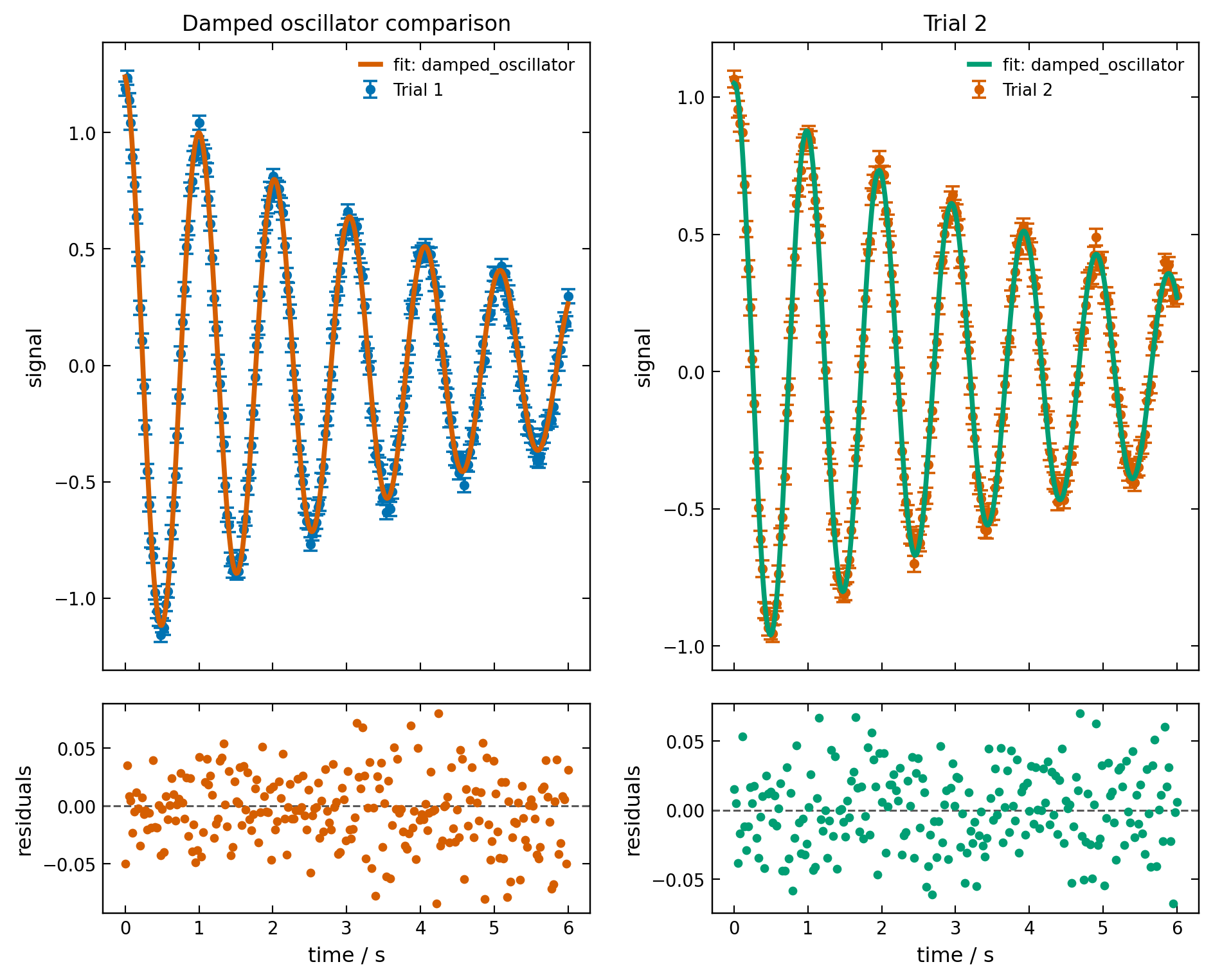
Side-by-side fit comparison with residual panels for each series.
Damped oscillator console output
Trial 1
  amplitude = 1.244714 ± 0.007525
  damping = 0.219231 ± 0.002599
  f = 0.980064 ± 0.000407
  phase = 0.096056 ± 0.006038
  reduced chi^2 = 1.065382
Trial 2
  amplitude = 1.051220 ± 0.006845
  damping = 0.183296 ± 0.002583
  f = 1.019614 ± 0.000429
  phase = -0.049326 ± 0.006753
  reduced chi^2 = 0.914054
Bimodal Gaussian fit
This example fits a sum of two Gaussian peaks using the built-in
bimodal_gaussian model.
import numpy as np
from labfit import fit, plot_fit

rng = np.random.default_rng(20260607)
x = np.linspace(-6.0, 10.0, 300)
y = (
    3.5 * np.exp(-0.5 * ((x - 0.0) / 0.9) ** 2)
    + 2.0 * np.exp(-0.5 * ((x - 4.5) / 1.2) ** 2)
    + rng.normal(0.0, 0.06, size=x.size)
)

result = fit(
    x, y, model="bimodal_gaussian",
    p0={"amplitude1": 3.0, "mean1": 0.0, "sigma1": 1.0,
        "amplitude2": 1.5, "mean2": 4.0, "sigma2": 1.0},
)
plot = plot_fit(result, show_residuals=True,
                title="Bimodal Gaussian fit")
plot.save("docs/_static/gallery/bimodal_gaussian.png")
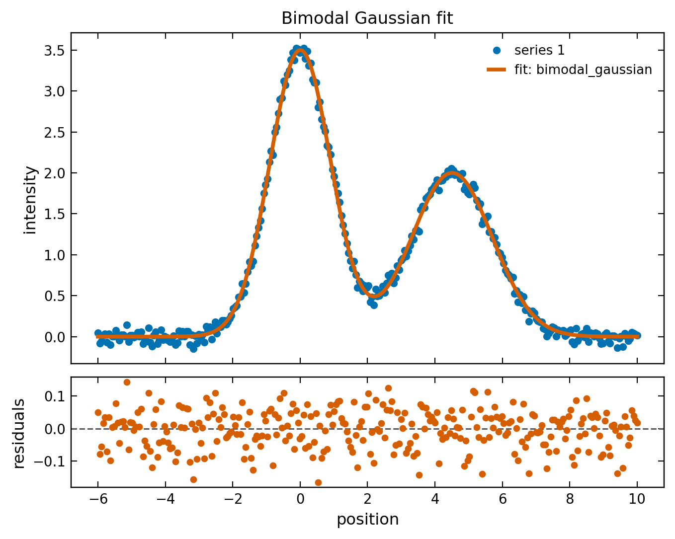
A two-peak Gaussian model fitted to synthetic data showing the fit curve and residuals.
Bimodal Gaussian fit console output
amplitude1 = 3.498592 ± 0.013417
mean1 = 0.003859 ± 0.004059
sigma1 = 0.902587 ± 0.004157
amplitude2 = 1.999901 ± 0.011716
mean2 = 4.508767 ± 0.008134
sigma2 = 1.195551 ± 0.008429
reduced chi^2 = 0.003556
Exponential decay with per-point errors
This example fits an exponential decay where every data point has its own y-uncertainty passed as an array. This is typical of counting-statistics experiments (radioactive decay, photon counts, etc.) where σ ∝ √(counts).
import numpy as np
from labfit import fit_curve, plot_fit

rng = np.random.default_rng(20260608)
x = np.linspace(0.0, 10.0, 40)

# True model: 5.0 * exp(-0.4 * x)
y_true = 5.0 * np.exp(-0.4 * x)

# Per-point uncertainties vary across the dataset
sigma = 0.05 + 0.08 * np.sqrt(y_true)
y = y_true + rng.normal(0.0, sigma)

result = fit_curve("exponential", x, y, sigma,
                   p0={"amplitude": 5.0, "decay": 0.5})
plot = plot_fit(result, show_residuals=True,
                title="Exponential decay with per-point errors",
                xlabel="time / s", ylabel="signal")
plot.save("docs/_static/gallery/exponential_fit.png")
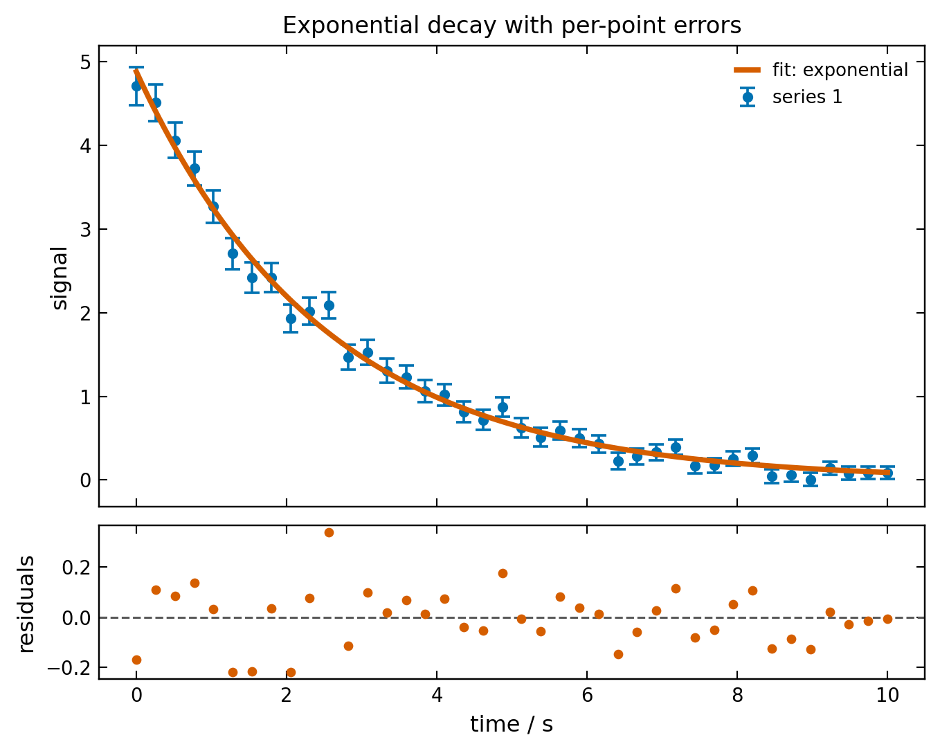
Each data point has its own uncertainty, shown by the error bars that vary in size across the dataset. The fit weights points accordingly.
Exponential fit console output
amplitude = 4.880850 ± 0.100131
decay = 0.399328 ± 0.008559
reduced chi^2 = 0.768797
Fitting a subset of your data
Fit only a region of interest (the peak) while plotting the full dataset, including the background. This is useful when your signal has a clear feature on top of a slowly-varying baseline.
import numpy as np
from labfit import fit_curve, plot_fit, Series

rng = np.random.default_rng(20260618)
x = np.linspace(0.0, 10.0, 300)
y = (3.0 * np.exp(-0.5 * ((x - 5.0) / 0.8) ** 2)
     + 0.05 * np.sin(1.5 * x)
     + rng.normal(0, 0.03, size=x.size))

full = Series(x=x, y=y, sigma=0.03, label="full data")

# Fit only the peak region
mask = (x > 3.5) & (x < 6.5)
result = fit_curve("gaussian", x[mask], y[mask], 0.03)

plot = plot_fit(result, data_series=full,
                title="Gaussian fit to peak region only")
plot.save("docs/_static/gallery/subset_fit.png")
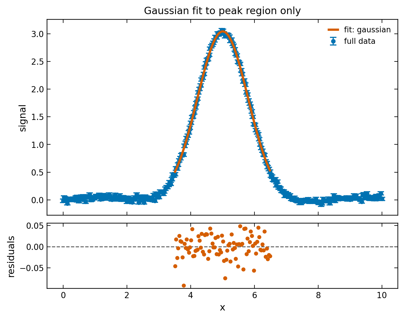
The fit was performed only on points with 3.5 < x < 6.5,
but the plot shows the full dataset with error bars.
Subset fit console output
amplitude = 3.044423 ± 0.005250
mean = 5.010007 ± 0.001580
sigma = 0.791448 ± 0.001760
reduced chi^2 = 0.805082
Comparing two models on the same data
Sometimes you are not sure which model is the right one. Fit the data with both and overlay the results on a single plot — the eye catches tail mismatches, and the reduced χ² confirms what you see.
Here the data comes from a Gaussian peak. The Gaussian fit (orange) recovers the parameters with χ² ≈ 1. The Lorentzian fit (green) is close near the centre but its heavier tails diverge from the data in the wings, giving χ² ≈ 17.
import numpy as np
from labfit import fit, plot_fit

rng = np.random.default_rng(20260620)
x = np.linspace(-4.0, 8.0, 200)
y_true = 5.0 * np.exp(-0.5 * ((x - 2.0) / 1.0) ** 2)
sigma = np.full_like(x, 0.08)
y = y_true + rng.normal(0.0, sigma)

# Correct model
result_gaussian = fit(x, y, model="gaussian", sigma=sigma, label="data")

# Close but wrong — Lorentzian has heavier tails
result_lorentzian = fit(x, y, model="lorentzian", sigma=sigma)

# Prevent the data markers from being drawn twice — only the
# Gaussian result carries the series so the points appear once.
result_lorentzian.series = None

plot = plot_fit(
    [result_gaussian, result_lorentzian],
    show_residuals=False,
    title="Gaussian vs Lorentzian model comparison",
    xlabel="position",
    ylabel="intensity",
)
plot.save("docs/_static/gallery/model_comparison.png")
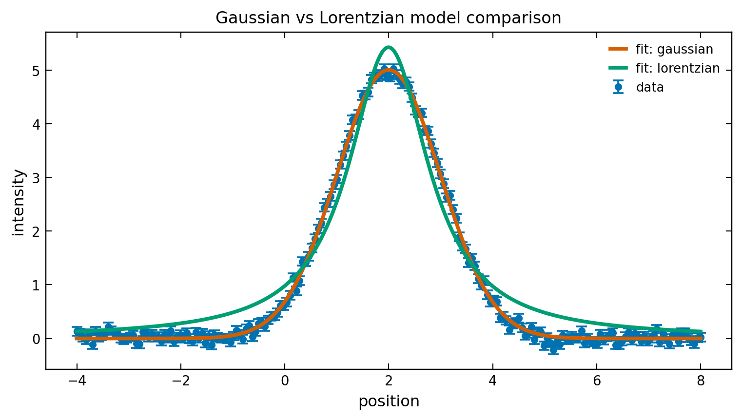
Both fit lines are drawn on the same axis. The Gaussian (orange) matches the data; the Lorentzian (green) deviates in the tails. The reduced χ² quantifies the difference: 1.07 vs 17.2.
Gaussian (correct model) console output
FitResult: gaussian
  amplitude = 5.0018 +/- 0.018636
  mean = 1.9985 +/- 0.004314
  sigma = 1.0027 +/- 0.004314
  reduced chi2 = 1.066
  p = 0.249
Lorentzian (close but wrong) console output
FitResult: lorentzian
  amplitude = 5.4251 +/- 0.095026
  center = 1.9966 +/- 0.016386
  gamma = 0.93677 +/- 0.023328
  reduced chi2 = 17.16  -- model may be wrong or errors underestimated
  p ~ 0.0e+00